

Author:
(1) Laurence Francis Lacey, Lacey Solutions Ltd, Skerries, County Dublin, Ireland.
Editor's Note: This is Part 4 of 7 of a study on how changes in the money supply, economic growth, and savings levels affect inflation. Read the rest below.
Table of Links
- Abstract and 1 Introduction
-
- Methods
- 2.1 Statistical Methodology
- 2.2 US Time Series Data
- 2.3 Hyperinflation Model
-
- Results
- 3.1 Characterisation of Price Inflation
- 3.2 Characterisation of Hyperinflation in the Weimar Republic (1922 to 1923)
- 4. Discussion
- 5. Conclusion, Supplementary materials, Acknowledgements, and References
- Appendix
3.1 Characterisation of Price Inflation
A plot of the natural log-transformed US BMS time series over the period 2001 to 2019 is given in Figure 1. The year 2001 is the reference year (time = 0), and the BMS data were expressed relative to the value obtained in year 2001. The corresponding plots for the natural log-transformed US CPI time series is given in Figure 2; the natural log-transformed US real GDP time series is given in Figure 3; the natural log-transformed average American household savings time series is given in Figure 4
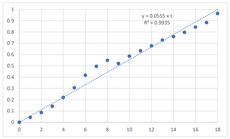
The average annual rate of growth of the US BMS, over the period 2001 to 2019, was 5.7%, with:
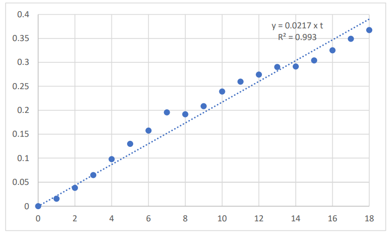
The average annual rate of US price inflation as measured by CPI, over the period 2001 to 2019, was 2.2%, with:
𝑣𝐶𝑃𝐼(𝑡) = 0.0217 x t
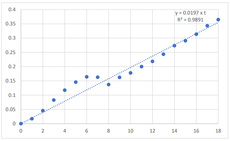
The average annual rate of growth of the US real GDP, over the period 2001 to 2019, was 2.0%, with:
𝑣𝐺𝐷𝑃(𝑡) = 0.0197 x t
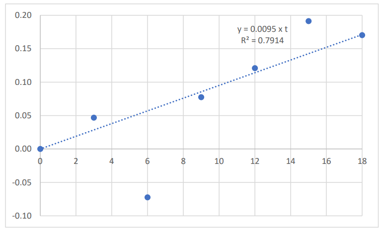
The average annual rate of growth of American household savings, over the period 2001 to 2019, was 1.0%, with:
𝑣𝑆𝐴𝑉(𝑡) = 0.0095 x t
The linear regression fits are summarised in Table 1.
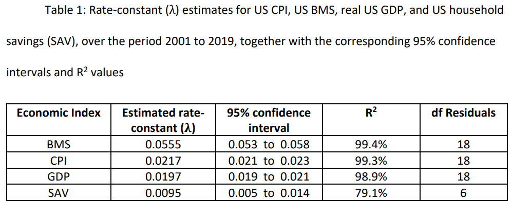
BMS, broad money supply; CPI, consumer price index; GDP, (real) gross domestic product; SAV, average American household savings; df, degrees of freedom
Henceforth, the annual US household savings estimates for the years not available were imputed, using the regression fit obtained from the available years of data.
The residual time series (RES(t)) was obtained from the relationship:
𝑅𝐸𝑆(𝑡) = 𝑣𝐵𝑀𝑆(𝑡) − 𝑣𝐺𝐷𝑃(𝑡) − 𝑣𝑆𝐴𝑉(𝑡) − 𝑣𝐶𝑃𝐼
This residual time series is plotted in Figure 5.
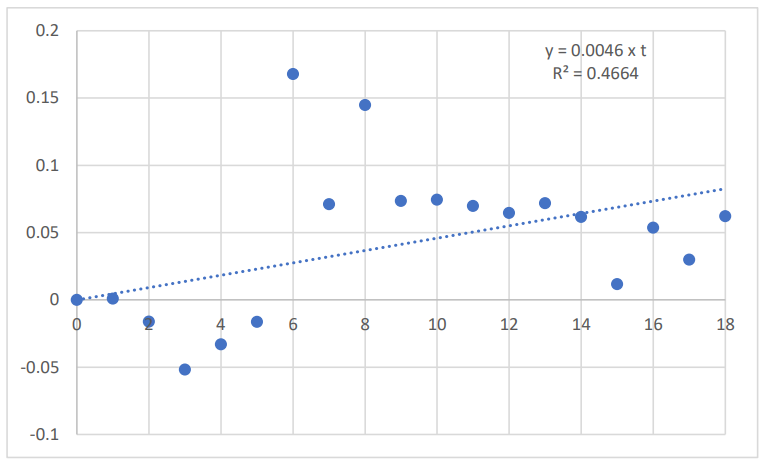
The average annual rate of growth of the residual time series (RES(t)), over the period 2001 to 2019, was 0.5%, with:
𝑅𝐸𝑆(𝑡) = 0.0046 x t
This gives:
𝑣𝐶𝑃𝐼(𝑡) = 𝑣𝐵𝑀𝑆(𝑡) − 𝑣𝐺𝐷𝑃(𝑡) − 𝑣𝑆𝐴𝑉(𝑡) − 𝑅𝐸𝑆(𝑡)
Further detail of the residual time series (RES(t)), over the period 2001 to 2019, are given in Table 2.
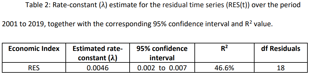
RES, residual time series; df, degrees of freedom
This paper is available on arxiv under CC BY-NC-ND 4.0 DEED license.